B树和B+树的定义以及应用
对于数据结构的学习,现在有些心得,就记录一下吧,想想自己当初学数据结构的时候,真是too young too simple。对于像红黑树,B树,B+树等数据结构,也许听上去很复杂,有点吓人,其实,我们所做的工作是利用好别人写好的代码,例如可以利用linux内核中的红黑树等数据结构,不需要造轮子,当然,如果有时间也可以自己动手写写,毕竟对自己也是一种提高麽!熟悉数据结构的应用场景,这点特别重要!接下来,我就放个大招了,哈哈,点开链接去看看吧,相信对你帮助巨大!!!大招链接
B-tree的定义
下面先说下B树的定义吧:
According to Knuth’s definition, a B-tree of order m is a tree which satisfies the following properties:
Every node has at most m children.
Every non-leaf node (except root) has at least ⌈m/2⌉ children.
The root has at least two children if it is not a leaf node.
A non-leaf node with k children contains k−1 keys.
All leaves appear in the same level
注:⌈m/2⌉是求大于m/2的最小整数值
上面是对m阶B树的定义,具体细节参考维基百科B树定义
4阶B-树更流行的称呼是2-3-4树,而3阶B-树叫做2-3树。
怎么样,是不是感觉很抽象,好,下面我将举一个例子,往3阶B树中依次插入整数1,2,3,4,5,6,7,8,然后再删除3,下面展示下结果
插入数据的结果如下图: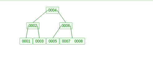
删除3后的结果如下图: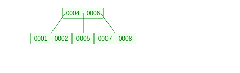
B+树的定义
B+树是一种特殊的B树,B+树与B树的区别如下:
B+ trees don’t store data pointer in interior nodes, they are ONLY stored in leaf nodes. This is not optional as in B-Tree. This means that interior nodes can fit more keys on block of memory.
The leaf nodes of B+ trees are linked, so doing a linear scan of all keys will requires just one pass through all the leaf nodes. A B tree, on the other hand, would require a traversal of every level in the tree. This property can be utilized for efficient search as well since data is stored only in leafs.
看到这里,也许读者们可能会感到困惑,好了,下面看看具体的示例吧。
分别往B树和B+中插入15,1,4,14,6,9,3,2,11,5,12,7,13,8,10。结果如下图:
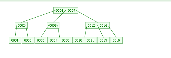
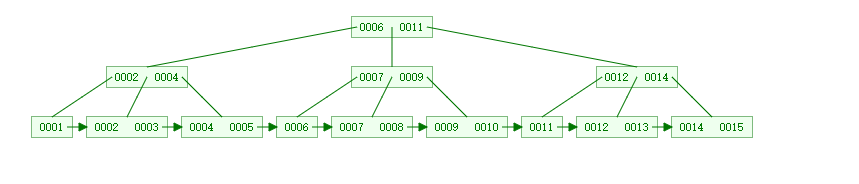
第一张图片为B树的结点情况,第二张图片为B+树的结点情况,此刻,对于B树和B+树的区别一目了然了吧。
B树与B+树的应用
看到一篇讲述B树和B+树特别好的一篇文章这里,怕自己的翻译水平误导到读者,故直接把原本搬过来,相信这篇文章觉得值得慢慢鉴赏。
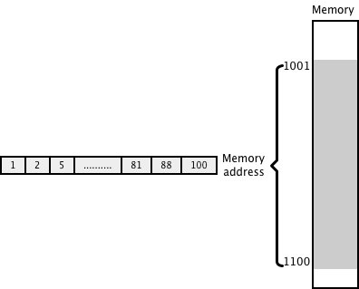
I love arrays because they are amazing data structures. Most languages allocate contiguous memory locations for an array thus they offer great memory locality. For accessing an element of an array, there is virtually no seek time required because elements are stored contiguously. With linked list, you never know where the next pointer is stored in memory, thus system might have to hop around quite a lot for locating a linked list node. This is very subtle distinction. Thus, while retrieving the elements of an array from disk, the access is super fast. To understand this better, lets understand how data is stored & accessed from external memory. Below diagram shows a glimpse of how data might be stored in memory:
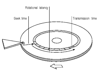
As you might have read, traditional HDD (Hard Disk Drive) has rotating drives which store data in tracks (parallel circular areas). When the data needs to be read or written, the actuator with an arm, needs to go to a particular sector on the track to read or write data. This is measured as seek time. After that, the drive needs to rotate to reach to a particular sector (rotational latency). This happens really fast but when we are reading huge amount of data, it might become a bottleneck since disk has to continuously move to specific sectors. Average seek times vary from 4ms for high end servers to 9ms for commonly used desktop drives.
SSD (Solid State Drive) offer superior performance because they have electrical connection for locating specific memory areas, rather then moving actuator with an arm. Thus, the access is very quick. But still, they also have average seek time of .10ms which might add up overtime for large data sets. Also, SSDs are expensive as compared to HDDs so not everyone is able to afford those.
I wanted to explain the process involved in fetching data from external memory perspective so that you can develop appreciation for memory locality. When we are accessing large data set and doing frequent read/write to/from disk, we need to consider this overhead. Based on type of disk, this can make your algorithm crawl. Anyways, since we now understand that memory locality is great for fast access, lets talk more about arrays.
As I said, arrays are fixed length data structures which offer great memory locality, but in real world, the size of the incoming data set cannot be predetermined. Also, if we store data arbitrarily in an array, we will have to do a linear scan to find a element. For large data sets stored in an array, two issues arise:
We don’t know the size of the data set in advance. If the data set size exceeds the preallocated size, we need to allocate bigger memory slot and copy old elements to new location. This is called dynamic array resizing.
Unless we keep data in some predefined order, searching will be really inefficient with O(n) worst case time for large data sets. If we keep data sorted, we can do efficient binary search to find items. But for large sorted data set, inserting new element will also require rearranging other elements which will be very inefficient. For small set, this should not be a big problem.
So looking at above two issues, it seem smaller fixed size sorted arrays are most efficient. But how this relates to use case where we have large data set? Well, we can break large data set into manageable small sorted arrays which can be efficiently searched. Also there has to be a way to link these different small sorted arrays with each other. Lets try it with an example. Assume that below array can’t be stored in one contiguous block of external memory:

We first try to sequentially break big array into multiple small ones as shown in below diagram. It seems like a singly linked list but with a caveat that each node has multiple keys. We can inspect the first & last element of each sub array and move forward until we reach to one which might have an element which we are looking for. Visualize doing this for large data set & how inefficient this linear search would be.

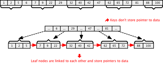
The other approach is to break array in ranges as shown in below diagram. Here we keep the top level array with few elements & the first sub array has elements less than the first element in the top array & so on. This is very similar to how we structure binary search tree but with two differences. Each parent node has more than one key and can point to more than two children. Also we can restrict on how many keys a particular node can have so that it doesn’t exceed allocated memory block [For example, 4 in below use case]. Here is an example:
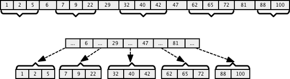
How will this improve efficiency? Well, if we keep this structure optimal, then while searching we can concentrate on one tree path which might have a particular element. For example, if we were to search for 22, we can do a linear search on top array (since array is small) and will figure out that a pointer between 6-29 must have our element. This means that we can virtually discard everything greater than equal to 29 since array is sorted. In technical terms, we are sub dividing search boundary to very small arrays at every step and eventually this would offer a logarithmic time. Feel it, this is really nice!
If you look at above diagram, we are trying to do following three things:
Every sub-array or node (for simplicity), should have pre defined maximum size. The size determines how many maximum keys can a node store. In above example it is 4.
If a node has k keys, then it can point to maximum (k+1) sub arrays. In our case, the top level array points to 5 sub-arrays, including ones before 6 and one after 81. This means that if an internal node has 3 child nodes (or sub-arrays) then it must have 2 keys: k1 and k2. All values in the leftmost sub-array will be less than k1, all values in the middle sub-array will be between k1 and k2, and all values in the rightmost sub-array will be greater than k2. The maximum number of child sub-arrays a node can point to is called order of the tree.
If we are dynamically creating this partitioning, then we need to make sure that each array has a minimum number of elements so that space is not wasted and our distribution doesn’t get skewed. This is a little more complicated than it sounds, since we need to split or merge sub-arrays if they have keys less than minimum number. That’s why keeping “structure optimal”, is essential.
Well, if you look at array tree diagram along with above properties, it essentially reflects the idea behind B-Tree. A linked sorted distributed range array with predefined sub array size which allows searches, sequential access, insertions, and deletions in logarithmic time. This structure is well suited for range queries as well. So lets formally define B-Tree now with some more properties:
A B-Tree of order k (children) is an k-ary search tree with the following properties:
The root node is either a leaf or has at least two children.
Each node, except for the root and the leaves, has between k/2 and k children. This is to make sure that tree is making optimal use of space and is not skewed.
Each path from the root to a leaf has the same length. In other words, all leaf are at same level. [This is something new but is needed to keep tree balanced]
The root, each internal node, and each leaf is typically a disk block. [For memory locality as explained above]
Each internal node has up to (k - 1) key values and up to k pointers to children, as k is the order of tree (order=maximum children).
The records are typically stored in leaves. In some cases, they are also stored in internal nodes.
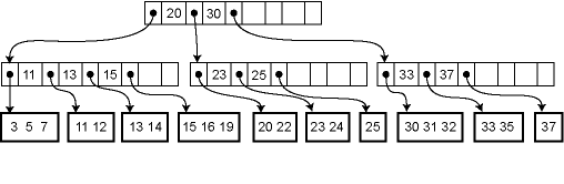
Here is a better hierarchical example:
B+ Trees are different from B Trees with following two properties:
B+ trees don’t store data pointer in interior nodes, they are ONLY stored in leaf nodes. This is not optional as in B-Tree. This means that interior nodes can fit more keys on block of memory and thus fan out better.
The leaf nodes of B+ trees are linked, so doing a linear scan of all keys will requires just one pass through all the leaf nodes. A B tree, on the other hand, would require a traversal of every level in the tree. This property can be utilized for efficient search as well, since data is stored only in leafs.
B+ trees are extensively used in both database and file systems because of the efficiency they provide to store and retrieve data from external memory. To understand indexing in a database, knowing about B and B+ trees is a pre requisite.
Consider this SQL & lets relate it to above structure:
select * from employees where salary between 100000 & 200000;
If we had created an index on salary, then we can find minimum bound in O(log n) time and then use the leaf linking property to scan through the elements until we reach to an element which is above 200000 (elements are sorted). If the leaf node size is big enough, then the range can be obtained very efficiently because of memory locality. If we had used binary search tree with some variant of in order traversal to find element between 100000 & 200000, it would not be as efficient as above. This is because of two reasons. One, because binary search tree have only two linked nodes & second, you can’t predict where the nodes are located in memory and thus have to hop a lot more in memory to extract the data. This technique is applicable to both RDBMS and key-value NoSql databases.
Thus B or B+ trees can be viewed as hierarchical index where root node represents the top level index. The insertion and deletion in a binary tree can trigger splitting or merging of a node(s) which I will cover in other post later. For now, sit back and appreciate the advantages which these data structures provide for accessing data from external memory while keeping data sorted. It is for this reason, they are used in both RDBMS and NoSql databases.
参考资料: